Automatically differentiating numerical integrators

Mar 9, 2022

JAX: Autograd and XLA

JAX is a research project from Google. For our purpose, JAX is a way to do automatic differentiation: With its updated version of Autograd, JAX can automatically differentiate native Python and NumPy functions. It can differentiate through loops, branches, recursion, and closures, and it can take derivatives of derivatives of derivatives. Numerical integration schemes are just native python and NumPy functions so JAX can automatically differentiate them. An example of when we might want to automatically differentiating numerical integrators is the control of nonlinear dynamical systems.

In particular, the purpose of this post is to learn how to do three things.

Use JAX.
Implement a few numerical integration schemes.
Use JAX to linearize a numerical integration scheme.

import jax.numpy as jnp
from jax import grad, jit, vmap, jacfwd, jacrev

import numpy as np
from tqdm.notebook import tqdm, trange

import matplotlib.pyplot as plt
from matplotlib.cm import ScalarMappable

Derivatives with JAX

JAX can compute derivatives through algorithms. A nice introduction is: https://www.assemblyai.com/blog/why-you-should-or-shouldnt-be-using-jax-in-2022/

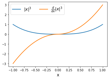
Here is a function, the rectified cube: \begin{equation} f(x) = |x|^3. \end{equation}

We can define $f(x)$ in a bit of a silly way by using an if statement.

def rectified_cube(x):
    r = 1
    if x < 0.:
        for i in range(3):
            r *= x
            r = -r
    else:
        for i in range(3):
            r *= x
    return r

JAX can differentiate this $f(x)$ no problem.

gradient_function = grad(rectified_cube)

fig, ax = plt.subplots(1)
xs = np.linspace(-1, 1)
fx = []
d_fx = []
for x in xs:
    fx.append(rectified_cube(x))
    d_fx.append(gradient_function(x))
ax.plot(xs, fx, xs, d_fx, lw=2)
ax.legend(['$|x|^3$', '$\\frac{d}{dx} |x|^3$'], fontsize=14, ncol=2)
ax.set_xlabel('x', fontsize=14);

Numerical integration + Autodiff

Here is a continuous model: \begin{equation} \dot{x}(t) = f(x(t), u(t)). \end{equation}

In many situations in computing (like model predictive control), the continuous dynamics must be converted to a discrete model \begin{equation} x_{k + 1} = F(x_k, u_k). \end{equation}

The reason for the conversion is that controls are computed as a zero-order-hold over discrete time intervals. The full discrete list of control amplitudes can be optimized. In the continuous limit, the discrete list becomes a function. Working with functions is much harder and doesn’t allow for a scheme like MPC which depends on taking a step. Plus, you can often use a simple basis to approximate function dynamics within the discrete time step (how?).

The RHS term $F(x_k, u_k)$ is a numerical integration. There are many ways to do this. $F$ is frequently nonlinear. Unfortunately, we really only know how to do MPC for systems with linear discrete dynamics where \begin{equation} F(x_k, u_k)=A x_k + B u_k. \end{equation} In order to do more interesting systems, we rely on locally linear approximations of $F$ in algorithms. This means the model is local about some guess trajectory, i.e. you compute matrices like \begin{equation} A \equiv \nabla_x F(x, u)|_{x_g} \end{equation} and multiply them with $x - x_g$ (it’s just the 1st order Fourier expansion). In MPC, the choice for $x_g$ (read: x-guess) is often a recently valid solution that’s been shifted to the left to accommodate the next prediction horizon. In any case, this means we want derivatives of $F$. This is where JAX comes in: If we know the continuous model $f$ and the algorithm $A$ we used to compute the numerical integration (i.e. $F = A \circ f$), we can find these linear approximations with automatic differentiaton.

Why might this be better? It’s hard (or at a minumum, annoying) to compute an analytic linearization of some numerical integrators $F$ even for simple nonlinear dynamics.

Exercise: Are there cases where it might not be reasonable to explicitely compute derivatives?

Van der Pol experiment

In this section, we’ll review some numerical integrators as preparation for thinking about how we might locally linearize them with JAX.

The toy system we will use is a driven Van der Pol oscillator, \begin{equation} \begin{aligned} &\dot{x}_1 = x_2, \
&\dot{x}_2 = -x_1 + \mu (1 - x_1^2) x_2 + u \end{aligned} \end{equation}

def vdp(t, x, u):
        mu = 2
        x1, x2 = x
        return jnp.array([
            x2,
            -x1 + mu * (1 - x1 ** 2) * x2 + u
        ])

Euler integration

The simplest choice for numerical integration is Euler integration, which combines the definition of the derivative \begin{equation} \dot{x}(t) = \lim_{\Delta t \rightarrow 0} \frac{\Delta x}{\Delta t} \end{equation} with the dynamics $\dot{x}(t) = f(t, x(t), u(t))$ such that \begin{equation} \frac{x_{k+1} - x_k}{\Delta t} \approx f(k, x_k, u_k) \end{equation} so \begin{equation} x_{k+1} \approx x_k + \Delta t f(k, x_k, u_k) \equiv F(x_k, u_k) \end{equation}

Set $z_k = [x_k, u_k]$ for simplicity.

def euler(z, dt=1):
    return z[:2] + dt * vdp(_, z[:2], z[2])

# Driving is external; set a policy.
def u_fn(t):
    return jnp.zeros_like(t)

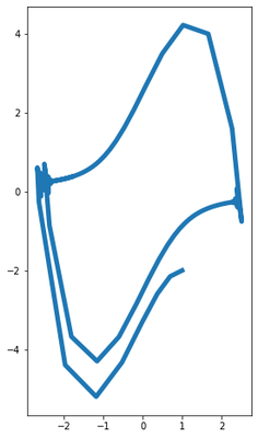
One fun thing to do is break the numerical integration by taking steps that are too big. Do that by dividing the interval [0,15] into 100 steps.

# Simulate the oscillator.
ts = jnp.linspace(0, 15, 100)
dt = ts[1] - ts[0]

t0 = ts[0]
x0 = jnp.array([[1], [-2]])

xs = [None] * (len(ts) + 1)
xs[0] = x0
for i, t in tqdm(enumerate(ts), total=len(ts)):
    z = jnp.vstack([xs[i], u_fn(t)])
    xs[i + 1] = euler(z, dt)
xs = jnp.hstack(xs)

x1, x2 = xs
fig, ax = plt.subplots(1, figsize=[8,8])
ax.plot(x1, x2, lw=5)
ax.set_aspect('equal')

We can compute the Jacobian of $F(x_k, u_k)$ using JAX. That is, we want to compute the derivative to arrive at a matrix, $\nabla_z F(z)$. There are a few ways to do this with JAX.

# Differentiate (retain ability to use other args)
jac_euler = jacfwd(euler)

# Is prefixing values faster? Not by much.
jac_euler_2 = jacfwd(lambda z: euler(z, dt))

# Is backward faster? No way! Recall: Why not?
jac_euler_3 = jacrev(euler)

jac_xs = [None] * len(ts)
det_jac_xs = [None] * len(ts)
for i, t in tqdm(enumerate(ts), total=len(ts)):
    z = jnp.vstack([xs[:, i][:, None], u_fn(t)])
    jac_xs[i] = jac_euler(z.squeeze(), dt)
    det_jac_xs[i] = np.linalg.det(jac_xs[i][:, :2])

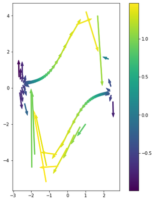
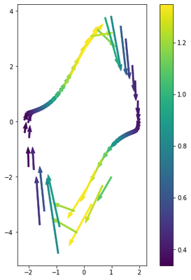
$\nabla_z F(z)$ is a matrix. Our goal in a first order linearization is to compute something like $\Delta F = \nabla_z F(z) \cdot \Delta z$. Here, let’s do that for the $x$ values.

# Find the differential of F
dx = xs[:, 1:] - xs[:, :-1]
df = np.vstack([jac_xs[i][:,:2] @ dx[:, i] for i in range(len(ts))]).T

Notice that the derivatives are only as good as our numerical integration (which we already decided to break). Keep in mind that this is the behavior you would get even if you did analytic derivatives with respect to the Euler integration scheme.

# Plot tangent vectors colored by the determinant of the Jacobian
fig, ax = plt.subplots(1, figsize=[8, 8])
cmap = plt.get_cmap('viridis')
norm = plt.Normalize(min(det_jac_xs), max(det_jac_xs))
for i in range(len(ts)):
    ax.arrow(x1[i], x2[i], df[0][i], df[1][i], width=.05,
             color=cmap(norm(det_jac_xs[i])))
ax.set_aspect('equal')
fig.colorbar(ScalarMappable(norm=norm, cmap=cmap))

If you want to peak at the matrix assoicated to $\nabla_z F(z)$, then you need to act on basis vectors.

basis = [None] * (xs.shape[0] + 1)
for i in range(len(basis)):
    basis[i] = np.zeros([xs.shape[0] + 1, 1])
    basis[i][i] = 1
    
z0 = jnp.vstack([xs[:, 0][:, None], u_fn(t)])
np.hstack([jac_euler(z0.squeeze(), dt) @ b for b in basis])

array([[1.        , 0.15151516, 0.        ],
       [1.0606061 , 1.        , 0.15151516]], dtype=float32)

Runge-Kutta methods

One nice thing with JAX is that if we pick more interesting numerical integration schemes, we don’t have to worry about computing the analytic derivative of the more complicated function $F(x_k, u_k)$. Let’s see this in action.

Generalize the Euler method so that \begin{equation} x_{k+1} \approx x_k + \Delta t \phi(k, x_k, u_k) \equiv F(x_k, u_k) \end{equation} with $\phi$ some new function defined to reduce errors by leveraging intermediate evaluations of $f$.

I’m not going to derive it, but one way to improve things is the classic 4th order Runge-Kutta:

\begin{equation} x_{k+1} \approx x_k + \frac{\Delta t}{6} (f_1 + 2 f_2 + 2 f_3 + f_4) \end{equation} where

$f_1 = f(t_k, x_k, u_k)$,

$f_2 = f(t_k + \Delta t / 2, x_k + f_1 \Delta t / 2, u_k)$,

$f_3 = f(t_k + \Delta t / 2, x_k + f_2 \Delta t / 2, u_k)$,

$f_4 = f(t_k + \Delta t, x_k + f_3 \Delta t, u_k)$.

Why do we modify the $x$ arguments in the function, but not the $u$ arguments? First off, we assume $f$ is a known function, but we don’t know anything about the control policy. Our control assumption is actually zero-order-hold so we are assuming $u_k$ won’t vary within our step. This is pretty important for the validity of the scheme. Luckily we’re in charge of the control so we can set this.

For completeness, let’s just say we don’t make the assumption of zero order hold. Then the Runge-Kutta approximation is not going to satisfy the promised accuracy, and we don’t have any way to improve the integration by cancelling Fourier terms like we did with $x$ (this is because $u$ is not constrained by a function). One final way to think about this: if we did know the policy, then $f(t, x, u) \mapsto f(t, x, \pi(t, x)) \equiv f^\pi(t, x)$ and we can have no gradients with respect to $u$ because it is fixed by the policy.

# Again, we don't have explicit time dependence. 
# Exercise: How would things change?
def rk4(z, dt=1):
    f1 = vdp(_, z[:2], z[2])
    f2 = vdp(_, z[:2] + f1 * dt / 2, z[2])
    f3 = vdp(_, z[:2] + f2 * dt / 2, z[2])
    f4 = vdp(_, z[:2] + f3 * dt, z[2])
    return z[:2] + (f1 + 2 * f2 + 2 * f3 + f4) * dt / 6

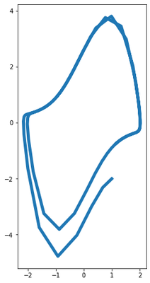
Pick the same time scheme as before, but now we’re going to get a much better numerical integration with our improved method.

# Simulate the oscillator.
xs = [None] * (len(ts) + 1)
xs[0] = x0
for i, t in tqdm(enumerate(ts), total=len(ts)):
    z = jnp.vstack([xs[i], u_fn(t)])
    xs[i + 1] = rk4(z, dt)
xs = jnp.hstack(xs)

x1, x2 = xs
fig, ax = plt.subplots(1, figsize=[8,8])
ax.plot(x1, x2, lw=5)
ax.set_aspect('equal')

Repeat the same differentiation process using JAX to get improved derivatives inherited directly from the improved numerical integration.

# Differentiate
jac_rk4 = jacfwd(rk4)

jac_xs = [None] * len(ts)
det_jac_xs = [None] * len(ts)
for i, t in tqdm(enumerate(ts), total=len(ts)):
    z = jnp.vstack([xs[:, i][:, None], u_fn(t)])
    jac_xs[i] = jac_rk4(z.squeeze(), dt)
    det_jac_xs[i] = np.linalg.det(jac_xs[i][:, :2])

  0%|          | 0/100 [00:00<?, ?it/s]

# Find the differential of F
dx = xs[:, 1:] - xs[:, :-1]
df = np.vstack([jac_xs[i][:,:2] @ dx[:, i] for i in range(len(ts))]).T

# Plot tangent vectors colored by the determinant of the Jacobian
fig, ax = plt.subplots(1, figsize=[8, 8])
cmap = plt.get_cmap('viridis')
norm = plt.Normalize(min(det_jac_xs), max(det_jac_xs))
for i in range(len(ts)):
    ax.arrow(x1[i], x2[i], df[0][i], df[1][i], width=.05,
             color=cmap(norm(det_jac_xs[i])))
ax.set_aspect('equal')
fig.colorbar(ScalarMappable(norm=norm, cmap=cmap))

Nice derivatives.

Control